Exploring Common Statistical Distributions

Statistics can seem like a complex subject, but at its heart, it’s about understanding how different things are spread out or distributed. Let’s break down some of the most common types of statistical distributions to make them more understandable.

Normal Distribution (Gaussian Distribution)

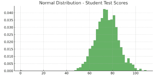
What It Is: Imagine a graph that’s bell-shaped and perfectly symmetrical. That’s a normal distribution used for things that vary around an average.
Key Feature: This distribution follows the 68-95-99.7 rule – about 68% of values are within 1 standard deviation from the mean, 95% within 2 standard deviations, and 99.7% within 3 standard deviations. In a normal distribution, this rule allows us to predict the likelihood of a data point falling within a certain range. This predictability is crucial in many fields, such as quality control, finance, and social sciences, where understanding the variability and predictability of data is essential.
When to Use: Great for continuous data that clusters around a mean. It’s common in natural and social sciences, especially with large samples.
Example: Imagine a high school where we are looking at students’ scores on a standardized math test. After compiling all the scores, we find that they form a normal distribution. The average (mean) score is 75 out of 100, with a standard deviation of 10 points.

• According to the Empirical Rule:
  • About 68% of the students scored between 65 (75 – 10) and 85 (75 + 10).
  • Around 95% scored between 55 (75 – 2×10) and 95 (75 + 2×10).
  • Nearly 99.7% scored between 45 (75 – 3×10) and 105 (75 + 3×10).
• This means most students scored close to the average, with fewer students obtaining very high or very low scores.

Binomial Distribution

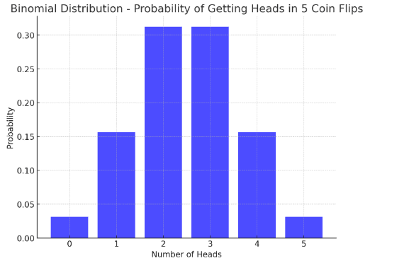
What It Is: This distribution counts the number of successes in a fixed number of trials. Each trial has only two possible outcomes – success or failure.
Key Feature: Useful when you’re dealing with two outcomes like yes/no, pass/fail, or win/lose.
When to Use: Perfect for situations with two outcomes like pass/fail. It’s used when you want to know the probability of a certain number of successes in a series of independent trials.
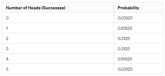
Example: Consider a game where a player flips a coin 5 times, and we count how many times the coin lands on heads (success). If the coin is fair, the probability of getting heads in a single flip is 0.5 (50%).

• If we define X as the number of heads (successes) in 5 flips, X follows a binomial distribution.
• The probability of getting exactly 3 heads, for example, can be calculated using the binomial formula.

Uniform Distribution

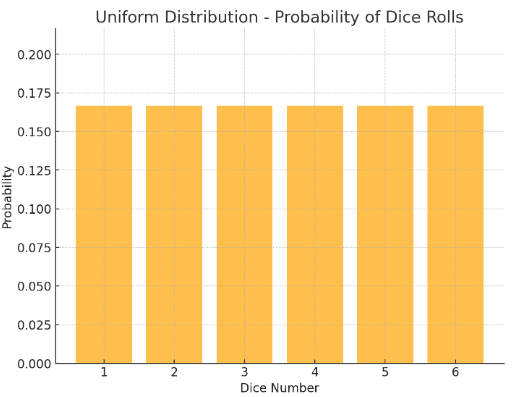
What It Is: All outcomes are equally likely to happen. Think of a perfectly flat line on a graph.
Example: Rolling a fair die. The outcomes 1, 2, 3, 4, 5, and 6 are all equally likely.
Key Feature: Every value between a minimum and maximum is just as likely as any other.
When to Use: If every outcome in a scenario is equally likely, like in simulations or games of chance, this is your go-to distribution.
Example: Let’s say we have a perfectly fair six-sided die. Each side, numbered 1 through 6, has an equal probability of landing face up.

• In this case, the probability of rolling any specific number (1, 2, 3, 4, 5, or 6) is exactly the same, 1/6.
• The uniform distribution here is discrete since there are a finite number of equally likely outcomes.

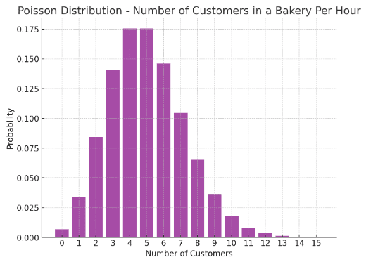
Poisson Distribution

What It Is: Used to count the number of times something happens over a set period or area.
Key Feature: Good for counting events, especially when they’re spread out randomly over time or space.
When to Use: When you’re counting the number of events in a set time or space and these events are independent of each other, like the number of emails you get in an hour.
Example: A small bakery observes the number of customers arriving during a particular hour every day. Let’s say they record an average of 5 customers per hour.

• If we let X be the number of customers arriving in an hour, X can be modeled by a Poisson distribution with a rate (λ) of 5 customers per hour.
• Using this model, the bakery can calculate probabilities for different numbers of customers arriving in an hour, like the probability of exactly 8 customers arriving.

Exponential Distribution

What It Is: It’s all about the time between events, especially when those events happen at a constant rate but independently of each other.
Key Feature: Often used to model waiting times or lifespans.
When to Use: Ideal for modeling the time until an event happens, like how long before a machine breaks down. It’s widely used in survival analysis and reliability engineering.
Example: A car rental service is analyzing the time between car maintenance appointments. They find out that, on average, a car needs maintenance every 50 days.

• Here, the time until a car needs maintenance follows an exponential distribution.
• With a mean time of 50 days, the service can estimate the probability of a car needing maintenance within a certain time frame, like within the next 30 days.

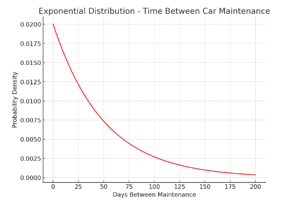
*The behavior of the exponential distribution might initially seem counterintuitive when thinking about the probability of events like car maintenance. However, it’s important to understand that the exponential distribution models the time until the next event (e.g., the need for maintenance) occurs, and it assumes that events happen independently of each other at a constant average rate.

Understanding these distributions can be super helpful in various fields, from science to economics. Each distribution has its unique characteristics and applications, making them valuable tools in your statistical toolbox. So, next time you’re faced with a data set, think about which distribution might best describe it!